This thread has been locked.

If you have a related question, please click the "Ask a related question" button in the top right corner. The newly created question will be automatically linked to this question.

[参考译文] MMWCAS-RF-EVM:方位角通道

Guru**** 2322270 points
Other Parts Discussed in Thread: MMWCAS-RF-EVM
请注意,本文内容源自机器翻译,可能存在语法或其它翻译错误,仅供参考。如需获取准确内容,请参阅链接中的英语原文或自行翻译。

https://e2e.ti.com/support/sensors-group/sensors/f/sensors-forum/1522795/mmwcas-rf-evm-azimuth-channels

部件号:MMWCAS-RF-EVM
主题: TX12中讨论的其他器件

工具/软件:

您好、

我将通读"使用4芯片级联的信号处理"文档、其中详细介绍了 MMWCAS-RF-EVM 并介绍了 TI 提供的 MATLAB 示例代码。 我正在仅使用级联雷达的方位角通道进行一些信号处理。 我对以下段落有疑问。  

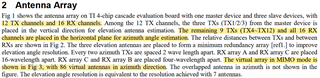
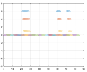
该文档指出使用 TX4~TX12和所有16RX 天线进行方位角处理。 然后、我们提到、由于忽略了重叠的天线、方位角方向上有86个虚拟天线。 因此、我想问是否有办法知道哪些天线对重叠、以便只能在我的处理中使用不重叠的86对 RX-TX? 另外、86个频道使用它们的顺序、如下图所示、在我的代码中按时间顺序使用它们。

提前感谢您的帮助!

  • 请注意,本文内容源自机器翻译,可能存在语法或其它翻译错误,仅供参考。如需获取准确内容,请参阅链接中的英语原文或自行翻译。

    您好、

    我们正在查看您的查询。 请允许我们在一天或两天内回复。

    此致

  • 请注意,本文内容源自机器翻译,可能存在语法或其它翻译错误,仅供参考。如需获取准确内容,请参阅链接中的英语原文或自行翻译。

    大家好、您能提供有关此方面的任何更新吗? 还有一个简短的后续问题、 方位平面(86个虚拟通道)上的每个虚拟 RxTx 对都相隔0.5个波长、还是该值不同?

  • 请注意,本文内容源自机器翻译,可能存在语法或其它翻译错误,仅供参考。如需获取准确内容,请参阅链接中的英语原文或自行翻译。

    尊敬的 Kauthar:

    有关天线 MMWCAS-RF-EVM 阵列(包括阵列中 AWR #s 的顺序和间距)的详细信息、请参阅"2.6.6虚拟天线阵列"AWR 用户指南(SWRU533A)部分。

    1.重叠的虚拟对不是显式的、但可以根据第0行中的 RX/TX 天线偏移和产生的天线阵列得出。  

    2.是的,每个虚拟通道间隔0.5波长。

  • 请注意,本文内容源自机器翻译,可能存在语法或其它翻译错误,仅供参考。如需获取准确内容,请参阅链接中的英语原文或自行翻译。

    感谢您的帮助! 我不确定是否正确、但我使用了 MATLAB 示例中提供的代码、这些代码列出了天线方向图。 我将其更改为具有 TXRX 标签、并使用标签沿 x 轴获取天线。 我仍然需要测试这种方法是否有效,但我在这里附加了代码,以防有人像我一样的问题。 谢谢。


    % TX and RX positions from TI cascade EVM
    TI_Cascade_TX_position_azi = [11 10 9 32 28 24 20 16 12 8 4 0];  % TX azimuth
    TI_Cascade_TX_position_ele = [6 4 1 0 0 0 0 0 0 0 0 0];          % TX elevation
    
    TI_Cascade_RX_position_ele = zeros(1,16); % RX elevation (azimuth plane)
    TI_Cascade_RX_position_azi = [11:14 50:53 46:49 0:3];           % RX azimuth
    TI_Cascade_RX_ID = [13 14 15 16 1 2 3 4 9 10 11 12 5 6 7 8];     % RX order
    
    TxToEnable = [12 11 10 9 8 7 6 5 4 3 2 1]; % TXs enabled (reversed index)
    D_TX = TI_Cascade_TX_position_azi(TxToEnable);
    D_TX_ele = TI_Cascade_TX_position_ele(TxToEnable);
    
    RxForMIMOProcess = TI_Cascade_RX_ID;
    D_RX = TI_Cascade_RX_position_azi(RxForMIMOProcess);
    D_RX_ele = TI_Cascade_RX_position_ele(RxForMIMOProcess);
    
    % TX/RX labels matching the board image
    tx_labels = {'TX12','TX11','TX10','TX9','TX8','TX7','TX6','TX5','TX4','TX3','TX2','TX1'};
    rx_labels = {'RX13','RX14','RX15','RX16','RX1','RX2','RX3','RX4', ...
                 'RX9','RX10','RX11','RX12','RX5','RX6','RX7','RX8'};
    
    %% FIGURE 1: Plot TX and RX antennas in physical order
    figure(1); clf; hold on; grid on;
    
    % Plot TX antennas with correct labels
    for i = 1:length(D_TX)
        plot(D_TX(i), D_TX_ele(i), 'rs', 'MarkerSize', 8, 'MarkerFaceColor', 'r');
        text(D_TX(i)+0.5, D_TX_ele(i)+0.3, tx_labels{i}, 'Color', 'r');
    end
    
    % Plot RX antennas with correct labels
    for j = 1:length(D_RX)
        plot(D_RX(j), D_RX_ele(j), 'g^', 'MarkerSize', 8, 'MarkerFaceColor', 'g');
        text(D_RX(j)+0.5, D_RX_ele(j)-0.5, rx_labels{j}, 'Color', 'g');
    end
    
    xlabel('Azimuth Position');
    ylabel('Elevation Position');
    title('Original TX/RX Antenna Geometry (Labeled by Physical Layout)');
    legend({'TX', 'RX'}, 'Location', 'best');
    ylim([-2 8]);
    
    %%
    % Virtual array generation with correct TX/RX labels
    figure(2); clf; hold on; grid on;
    
    % TX and RX positions (already defined)
    % D_TX, D_TX_ele, D_RX, D_RX_ele, tx_labels, rx_labels
    
    % Arrays to store points and labels
    RX_id_tot = [];
    RX_id_tot_ele = [];
    txrx_labels = {};
    h_points = [];
    
    for ii = 1:length(D_TX)
        for jj = 1:length(D_RX)
            % Virtual antenna coordinates
            RX_id_new = D_RX(jj) + D_TX(ii);
            RX_id_new_ele = D_RX_ele(jj) + D_TX_ele(ii);
    
            % Store coordinates
            RX_id_tot(end+1) = RX_id_new;
            RX_id_tot_ele(end+1) = RX_id_new_ele;
    
            % Store label using correct TX/RX physical labels
            txrx_labels{end+1} = sprintf('%s–%s', tx_labels{ii}, rx_labels{jj});
    
            % Plot the point
            h = plot(RX_id_new, RX_id_new_ele, 'bo', 'MarkerSize', 6, 'MarkerFaceColor', 'b');
            h_points(end+1) = h;
        end
    end
    
    % Store label data in UserData for interactive labeling
    for k = 1:length(h_points)
        set(h_points(k), 'UserData', txrx_labels{k});
    end
    
    % Enable interactive data cursor mode
    dcm = datacursormode(gcf);
    set(dcm, 'Enable', 'on', 'UpdateFcn', @customDataTip);
    
    xlabel('Azimuth Coordinate');
    ylabel('Elevation Coordinate');
    title('Virtual Antenna Array — Click Dot to View TX–RX Pair');
    ylim([-2 10]);
    
    % Custom data cursor callback function
    function output_txt = customDataTip(~, event_obj)
        hTarget = get(event_obj, 'Target');
        label = get(hTarget, 'UserData');
        pos = get(event_obj, 'Position');
        output_txt = {['X: ', num2str(pos(1))], ...
                      ['Y: ', num2str(pos(2))], ...
                       label};
    end